使用Open SAR Toolkit进行哨兵1号数据的自动化预处理

Open SAR Toolkit(OST)是一个用于Sentinel-1数据预处理的Python包，支持Sentinel-1分析就绪数据(Analysis Ready Data, ARD)的自动生成。OST最初由联合国粮食及农业组织（FAO）开发，现在由ESA负责。

安装依赖项

安装配置SNAP

SNAP是OST的依赖软件。首先在此处下载安装包并安装SNAP。

配置SNAP python环境（可选）

SNAP本身也是提供Python接口的。关于SNAP支持的Python版本。SNAP Wiki的说法是2.7和3.3~3.6，但SNAP安装时的提示Only Python versions 2.7, 3.3 and 3.4 are supported。
OST支持的的Python版本为>=3.5。

考虑到以后可能会用到SNAP Python接口，暂且采用SNAP Wiki的说法，在conda创建了python 3.6环境用来配置SNAP和OST。

conda create -n py36 python=3.6
conda activate py36

安装过程参考SNAP Wiki。

安装过程中没有检查到python环境，所以没有选择。安装完成后再手动配置。

snap/bin/snappy-conf <python-exe>

如果不知道自己的python解释器位置，通过where python（Window）或which python（Linux）查看

因此对我来说，该命令为

sh snappy-conf /home/fangzhe/anaconda3/envs/py36/bin/python3.6

配置完毕后的信息：

/home/fangzhe/snap/bin/../platform/lib/nbexec: WARNING: environment variable DISPLAY is not set
Configuring SNAP-Python interface…
Done. The SNAP-Python interface is located in ‘/home/fangzhe/.snap/snap-python/snappy’
When using SNAP from Python, either do: sys.path.append(‘/home/fangzhe/.snap/snap-python’)
or copy the ‘snappy’ module into your Python’s ‘site-packages’ directory.

根据该消息，手动将’/home/fangzhe/.snap/snap-python/snappy’复制到/home/fangzhe/anaconda3/envs/py36/lib/python3.6/site-packages

配置完毕后可以使用以下代码进行测试：

from snappy import ProductIO
import numpy as np
import matplotlib.pyplot as plt
 
p = ProductIO.readProduct('snappy/testdata/MER_FRS_L1B_SUBSET.dim')
rad13 = p.getBand('radiance_13')
w = rad13.getRasterWidth()
h = rad13.getRasterHeight()
rad13_data = np.zeros(w * h, np.float32)
rad13.readPixels(0, 0, w, h, rad13_data)
p.dispose()
rad13_data.shape = h, w
imgplot = plt.imshow(rad13_data)
imgplot.write_png('radiance_13.png')

安装Orfeo Toolbox（可选）

OST的影像镶嵌功能依赖于Orfeo Toolbox的otbcli_Mosaic命令，因此如果想使用镶嵌功能需要下载安装Orfeo Toolbox。

安装后确保安装目录下的bin目录设置到了PATH环境变量。

安装OST

方法：通过conda安装

首先安装依赖包

conda install pip gdal jupyter jupyterlab git matplotlib numpy rasterio imageio rtree geopandas fiona shapely matplotlib descartes tqdm scipy joblib retrying pytest pytest-cov nodejs

# this is needed for the progress bar when downloading
jupyter labextension install @jupyter-widgets/jupyterlab-manager
jupyter nbextension enable --py widgetsnbextension

然后安装OST

pip install git+https://github.com/ESA-PhiLab/OpenSarToolkit.git

未解决：Windows下使用报错

注意OST是依赖snap的，需要提供 SNAP gpt命令行exe文件路径(e.g. C:\path\to\snap\bin\gpt.exe)

数据处理

OST没有提供文档，代码也基本没有注释，学习时主要参考ESA提供的一份Jupyter notebook教程。不过该教程版本较老，很多类和函数的名字和参数有所变动，需要查看源码自行订正。

from ost import Sentinel1Scene

scene_id = 'S1A_IW_GRDH_1SDV_20191116T170638_20191116T170703_029939_036AAB_070F'
# create an S1Scene instance
s1 = Sentinel1Scene(scene_id)

# 查看数据基本信息
print(s1.info())

# 数据下载（需要输入NASA Earthdata的账号和密码）
output_dir = 'your path'
s1.download(output_dir)

# 数据预处理
s1.create_ard(infile, output_dir)

讨论

OST做了哪些预处理工作

Sentinel1Scene的构造函数__init__(self, scene_id, ard_type='OST_GTC', log_level=logging.INFO)需要一个分析就绪数据类型，默认为OST-GTC。其他几种类型分别为CEOS、Earth-Engine、OST-RTC（jupyter notebook上讲的过期了）。

Sentinel1Scene.create_ard()函数可实现Analysis Ready Data(ARD)的自动生成（仅支持GRD产品，不支持SLC产品），通过追踪源码，可知主要由grd_to_ard.grd_to_ard(filelist, config_file)实现，我们以OST-GTC类型为例，查看具体的处理步骤：

1. 导入数据, 关键函数为grd_wrappers.grd_frame_import()，用于更新轨道信息(orbit information)，移除热噪声(thermal noise)。
2. 移除边缘噪声(border noise), if ard[‘remove_border_noise’] and not subset。
3. 辐射校正（calibration）
4. 多视（multi-look），将每个像元的地面分辨率修正为长宽一致if int(ard[‘resolution’]) >= 20，默认执行。多视处理的目的是为了抑制斑点噪声，但同时会降低分辨率。
5. Layover shadow mask：为具有重叠效应（layover effect）和阴影效应（shadow effect）的地区创建掩膜（if ard[‘create_ls_mask’] is True，默认不执行）如果执行该处理，会在输出文件目录下生成*_ls_mask.json，内容为geojson格式的掩膜。
6. 斑点噪声滤波（Speckle filtering）（if ard[‘remove_speckle’]），默认不做，猜测是因为多视处理已经做了噪声抑制。如果做的话默认使用 Refined Lee 滤波算法。
7. 如果要生成的产品类型OST-RTC，执行Terrain flattening，Terrain flattening的效果可见下文。
8. Linear to db，默认不做
9. Geocoding：执行地形校正（Terrain Correction）
10. Create an outline：在输出目录生成*_bounds.json，内容为geojson格式的影像边界

OST是怎么确定执行哪些步骤的

生成ARD过程中所依据的处理参数来自processing.json，由Sentinel1Scene.get_ard_parameters()函数生成：

def get_ard_parameters(self, ard_type):

    # find respective template for selected ARD type
    template_file = OST_ROOT.joinpath(
        f"graphs/ard_json/"
        f"{self.product_type.lower()}."
        f"{ard_type.replace('-', '_').lower()}.json"
    )
    # open and load parameters
    with open(template_file, 'r') as ard_file:
        self.ard_parameters = json.load(ard_file)['processing']

由get_ard_parameters()可知，配置参数的模板文件位于 ost根目录/grahps/ard_json，打开该路径，可以发现一共有7个模板文件：

• grd.ceos.json
• grd.earth_engine.json
• grd.ost_gtc.json
• grd.ost_rtc.json
• slc.ost_gtc.json
• slc.ost_minimal.json
• slc.ost_rtc.json

很明显，前4个模板分别对应4种产品类型。

打开比较一下有何不同，

Earth-Engine: "resolution": 10,"product_type": "GTC-sigma0"

CEOS: "resolution": 10,"product_type": "RTC-gamma0","create_ls_mask": true

OST-RTC: "product_type": "RTC-gamma0", "create_ls_mask": true,

在处理过程中，OTC与GTC最大的区别就是OTC执行

Earth-Engine的分辨率是OST-GTC的2倍，最后的数据体积也是OST-GTC的2倍。Earth-Engine的结果特别奇怪，处理的一个数据结果分布基本是(-0.5, 0.5)但尾巴特别长，总体数据范围为(-120, 11067)。不知道是数据的问题还是这种产品都是这样的。

附上OST-GTC的参数文件：

{
    "processing": {
        "single_ARD": {
            "image_type": "GRD",
            "ard_type": "OST-GTC",
            "resolution": 20,
            "remove_border_noise": true,
            "product_type": "GTC-gamma0",
            "polarisation": "VV, VH, HH, HV",
            "to_db": false,
            "to_tif": false,
            "geocoding": "terrain",
            "remove_speckle": false,
            "speckle_filter": {
                "filter": "Refined Lee",
                "ENL": 1,
                "estimate_ENL": true,
                "sigma": 0.9,
                "filter_x_size": 3,
                "filter_y_size": 3,
                "window_size": "7x7",
                "target_window_size": "3x3",
                "num_of_looks": 1,
                "damping": 2,
                "pan_size": 50
            },
            "create_ls_mask": false,
            "apply_ls_mask": false,
            "dem": {
                "dem_name": "SRTM 1Sec HGT",
                "dem_file": "",
                "dem_nodata": 0,
                "dem_resampling": "BILINEAR_INTERPOLATION",
                "image_resampling": "BICUBIC_INTERPOLATION",
                "egm_correction": false,
                "out_projection": 4326
            } 
        },
        "time-series_ARD": {
            "to_db": true,
            "remove_mt_speckle": true,
            "apply_ls_mask": false,
            "mt_speckle_filter": {
                "filter": "Refined Lee",
                "ENL": 1,
                "estimate_ENL": true,
                "sigma": 0.9,
                "filter_x_size": 3,
                "filter_y_size": 3,
                "window_size": "7x7",
                "target_window_size": "3x3",
                "num_of_looks": 1,
                "damping": 2,
                "pan_size": 50
            },
            "apply_ls_mask": false,
            "deseasonalize": false,
            "dtype_output": "float32"
        },
        "time-scan_ARD": {
            "metrics": ["avg", "max", "min", "std", "cov"],
            "remove_outliers": true,
            "apply_ls_mask": false
        },
        "mosaic": {
            "harmonization": true,
            "production": false,
            "cut_to_aoi": true
        }
    }
}

应该该采用哪种预处理方案

除了不同的ARD类型有不同的处理步骤，其他教程也有不同的预处理方案，网上大部分的教程，包括ESA的官方教程和ASF的官方教程，都只执行了如下三个步骤（省略轨道信息更新和图像裁剪）。

1. Calibration
2. Speckle Filtering
3. Terrain Correction（Range-Doppler Terrain Correction）

关于这个问题，在OST的Github仓库提交了一个issue，向作者请教，作者的回复如下：

……Now for your case of flood mapping, GTC products are sufficient, since you do not expect floods on slopes. In general, and as a one-size-fits-all ARD type, I recommend OST-RTC, which includes the terrain flattening and the ARD is suitable as well for other types of land cover mapping, or bio-geophysical parameter retrieval.

总的来说，在洪涝提取中，GTC产品就足够了。如果说需要一种适合所有场景的ARD类型，作者更推荐OTC。OTC和GTC最主要的区别是OTC执行了Terrain flatting，纠正山体起伏造成的坡向的辐射。下面两张图是一个很好的例子：

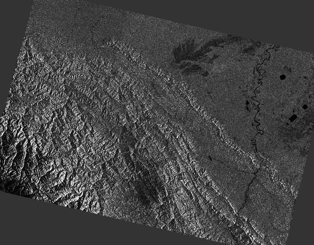
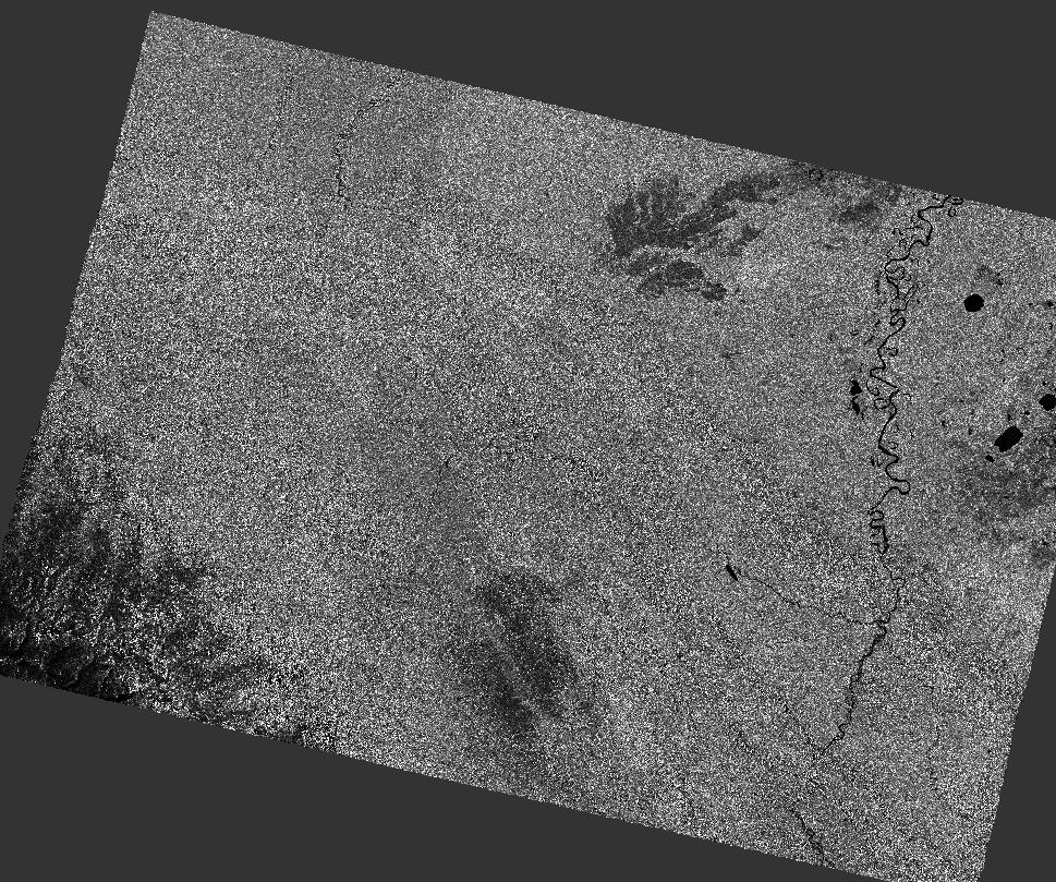
上图为默认OST-GTC参数得到的结果，下图为默认OST-RTC参数得到的结果。数据为，可以很明显地看出Terrain Flatting消除了地形起伏的影响。

综合考虑这些信息，采用以下配置方法：ard_type为OST-RTC以执行terrain flatting，除默认预处理步骤，增加斑点噪声滤波和dB化两个步骤。代码如下所示：

s1 = Sentinel1Scene(scene_id, 'OST-RTC')
s1.ard_parameters['single_ARD']['remove_speckle'] = True
s1.ard_parameters['single_ARD']['to_db'] = True
output_dir = output_dir_base + '/My-Param'
s1.create_ard(infile, output_dir)

输出数据的格式

处理结果为SNAP推荐的BEAM-DIMAP格式，记录了地理编码、文件占用、尺寸、成像日期、传感器类型等元数据，该格式的具体说明摸这里。SNAP称其是唯一一种正确存储所有元数据的格式。如果将其导出为Geotiff等格式，会丢失很多信息。

SNAP的建议是，尽量使用BEAM DIMAP格式，只有在SNAP中的数据处理结束的时候才导出为其他数据格式。如果想在外部软件读取一个栅格，可以打开.data目录，里面有所有栅格的img格式和hdr头文件。

如果想直接输出tif格式，可以修改配置参数，见下文。

自定义处理内容

通过修改配置参数，可以对处理过程进行自定义。

（1）官方的一个示例，修改分辨率和重采样方法

s1.ard_parameters['single ARD']['resolution'] = 50
s1.ard_parameters['single ARD']['dem']['image resampling'] = 'BILINEAR_INTERPOLATION'

（2）由于OST默认不做to db，可以修改to db参数：

s1.ard_parameters['single_ARD']['to_db'] = True  # 要求转为db

（3）斑点噪声滤波

s1.ard_parameters['single_ARD']['remove_speckle'] = True

（3）只输出VV波段：

s1.ard_parameters['single_ARD']['polarisation'] = 'VV'

（4）将输出格式改为Geotiff

s1.ard_parameters['single_ARD']['to_tif'] = True

报错了：TypeError: in method ‘wrapper_GDALWarpDestDS’, argument 1 of type ‘GDALDatasetShadow *’，懒得探究原因了，用GDAL自己转吧。

斑点噪声滤波的效果

先看一下数据处理的效果：上图是没做滤波，下图做了滤波。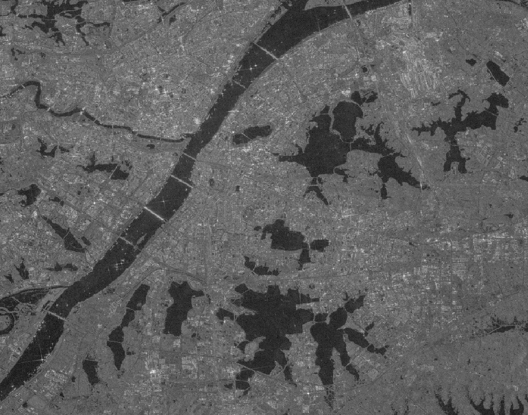

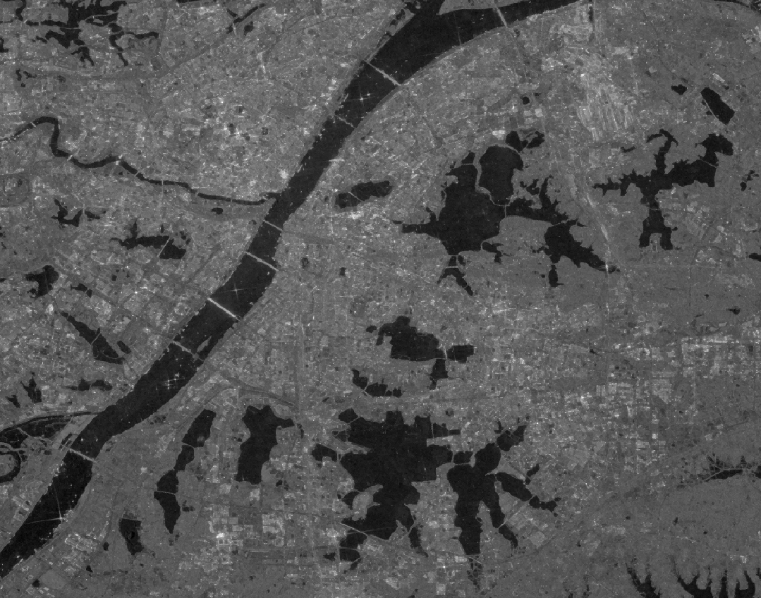
（需要放大才能看清），不做滤波的话，建筑的边界还是比较明显的，做了滤波之后就没有那么明显了。

来看一下水体提取的效果。使用经典的Otsu阈值分割算法提取水体，上图是没有做滤波的，下图是做了滤波的。

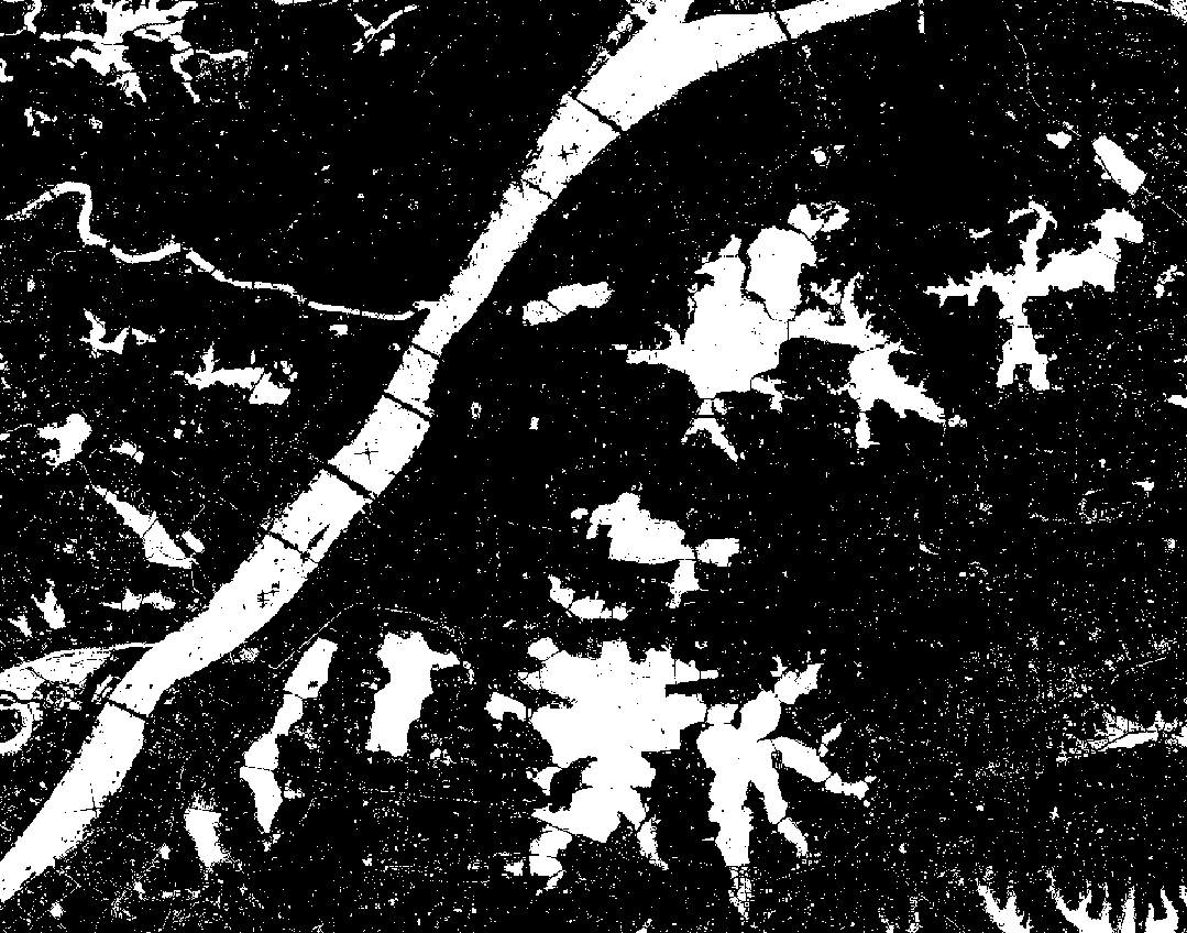
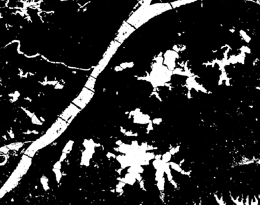
效果非常明显，斑点噪声滤波去除了绝大部分的噪点，因此一部分空间分辨率的损失是值得接受的。

其他问题

SAR数据的单位，gamma0与sigma0的区别？

Earth-Engine的输单位出为sigma0, OST-GTC为gamma0

‘apply_ls_mask’参数似乎并不会起作用

追踪代码时发现并没有用到ard[‘apply_ls_mask’]，配置ard['apply_ls_mask'] = True好像也并没有效果

其他参考

ASF Data Recipe (Tutorials):
asf.alaska.edu/how-to/data-recipes/data-recipe-tutorials/

Layover-Shadow Mask Generation

摘自SNAP帮助文档

This operator can also generate layover-shadow mask for the orthorectified image. The layover effect is caused by the fact that the signal backscattered from the top of the mountain is actually received earlier than the signal from the bottom, i.e. the fore slope is reversed. The shadow effect is caused by the fact that no information is received from the back slope. This operator generates the layover-shadow mask as a separate band using the 2-pass algorithm given in section 7.4 in [2]. The value coding for the layover-shadow mask is defined as the follows:

• corresponding image pixel is not in layover, nor shadow
• corresponding image pixel is in layover
• corresponding image pixel is in shadow
• corresponding image pixel is in layover and shadow
• User can select output the layover-shadow mask by checkmarking “Save Layove-Shadow Mask as band” box in SAR-Simulation tab.

To visualize the layover-shadow mask, user can bring up the orthorectified image first, then go to layer manager and add the layover-shadow mask band as a layer.